
I haven’t explored ray tracing and path tracing techniques in a while. Recently, I stumbled upon this cool workshop that got me excited about diving back into the topic. It’s a chance for me to approach path tracing and its implementation in a whole new way and document my journey along the process. :)
In this post I will follow the structure of the workshop - as it provides a clear and less overwhelming roadmap - to document one of the perspectives / implementations of path tracing. I will refer to books and articles I’ve explored to expand parts that are important or interesting, and note down those deeper topics to cover in the future.
- About the Workshop
- On Ray Tracing
- On Path tracing
- Progressive rendering on Shadertoy
- Final Thoughts
About the Workshop
This workshop shows how to:
- Implement ray tracing in software on the GPU.
- Use GLSL, Shadertoy, camera models, ray-triangle intersection tests, and ray-mesh intersection tests.
- Build on your ray tracer and implement a path tracer that renders a scene with full global illumination.
- Learn about fundamental concepts in physically based rendering such as global illumination, radiance, the rendering equation, Monte Carlo integration, and path tracing.
- Implement the Monte Carlo integration, and use it to compute direct illumination.
- Write your path tracer.
And it contains:
- Framework provided - shadertoy etc.
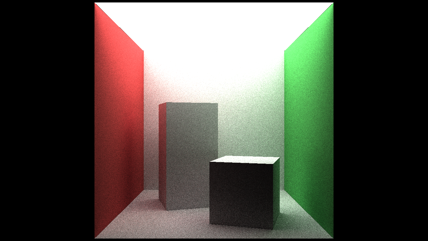
- Scene provided - triangles only cornell box
- Only diffuse surface
- no textures
- no acceleration structures - bvh
- no clever sampling / denoising
- running on GPUs because GLSL, so no graphics APIs
More about the workshop from the author can be found on his blog.
On Ray Tracing
A tiny ray tracer
Firstly, start with a fun trivia: Back of the Business Card Ray Tracers

Ray tracing vs Path tracing?
Then we need to clarify terms that are constantly misused in various contexts:
- Ray tracing is a technique for modeling light transport for use in a wide variety of rendering algorithms (esp. Path tracing) for generating digital images. It’s the foundation of path tracing.
- Path tracing is a Monte Carlo method of rendering images of 3D scenes such that the global illumination is faithful to reality. Path tracing is using ray tracing technique.
Because ray tracing is so incredibly simple, it should have been an obvious choice for implementing global illumination in computer graphics. – A Ray-Tracing Pioneer Explains How He Stumbled into Global Illumination, a good read by J. Turner Whitted
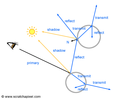
Ray tracing itself is sufficient to produce interesting renders – like the Whitted Ray Tracing algorithm, but the result will not be a physically accurate render that has global illumination, which is where path tracing come into play.
No matter what, the Whitted algorithm is still the classical example of an algorithm that uses ray tracing to produce photo-realistic computer-generated images. Even though we can see the result is very CG-like:
More articles on the topic:
- Overview of the Ray-Tracing Rendering Technique
- Light Transport Algorithms and Ray-Tracing: Whitted Ray-Tracing
- An Integrator for Whitted Ray Tracing - pbrt
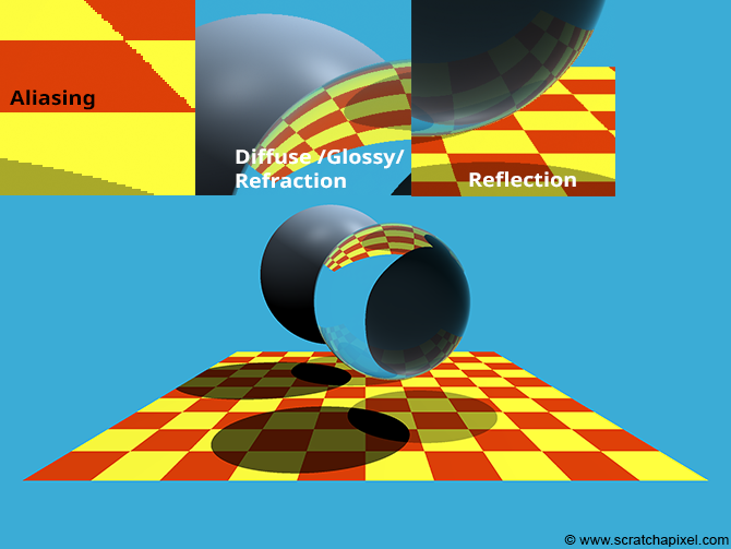
What effects are captured by path tracing that are not captured by ray tracing? Here is one of the best explaination I came across:
Generally speaking, path tracing removes a number of assumptions that ray tracing makes.
- Ray tracing usually assumes that there is no indirect lighting (or that indirect lighting can be approximated by a constant function), because handling indirect lighting would require casting many additional rays whenever you shade an intersection point.
- Ray tracing usually assumes that there is no non-glossy reflection (or called diffuse reflection), because while it is fairly easy to handle glossy/mirror reflection (you reflect the ray and continue with the ray tracing), if you have non-glossy specular reflection you have a problem very much like indirect lighting: you need to trace a bunch more rays and then do lighting wherever those rays hit.
- Ray tracing also usually assumes that there are no area lights, because it is very cheap to cast a single ray towards a light to determine if an intersection point is in shadow, but if you have an area light you generally need to cast multiple rays towards different points on the area light to determine the amount that the intersection point is shadowed.
- And as soon as you need to break any of those assumptions with ray tracing, you now have a sampling problem: you need to decide how to distribute the many additional rays you need to trace in order to get an accurate result that doesn’t have noticeable aliasing.

More articles on the topic:
GLSL refresher
Features
- C-like shader language for OpenGL, Vulkan, WebGL
- For-loops of fixed max_length, no while-loops
- Fixed-size arrays, no pointers
- Indices must be constants
Syntax
-
Parameters in functions can be marked
in,outorinout, copy values in, out or both Built-in scalar, vector, matrix types: int float - Built-in scalar, vector and matrix types:
int float vec2 vec3 vec4 mat2 mat3
- Constructor-like functions:
vec3 v = vec3(x, y, z);mat3 A = mat3(col_0, col_1, col_2);
- Standard functions/operators for geometric operations:
dot (v, w)
- Swizzles and array operators:
vec2(v[ ], v[ ]) == v.yzv.xyz == v.rgbfloat col_1_row_2 = A[1][2];
Scene representation
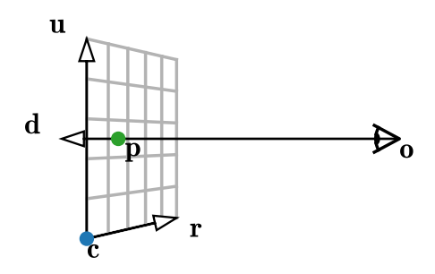
- Camera - generate camera ray, or
get_primary_ray_direction() - Triangle - 3D geometry with surface material info
- Mesh - Many triangles
Camera
Shape - Triangle
Triangle definition. Here it contains both geo data and surface data, for simplicity.
In better implementation like in pbrt, geo data is the only focus for shape class, and a material class will focus on surface data including a reference to texture class. Above all, a primitive class will encompass both shape and material.
// A triangle along with some shading parameters
struct triangle_t {
    // The positions of the three vertices (v_0, v_1, v_2)
    vec3 positions[3];
    // A vector of length 1, orthogonal to the triangle (n)
    vec3 normal;
    // The albedo of the triangle (i.e. the fraction of
    // red/green/blue light that gets reflected) (a)
    vec3 color;
    // The radiance emitted by the triangle (for light sources) (L_e)
    vec3 emission;
};
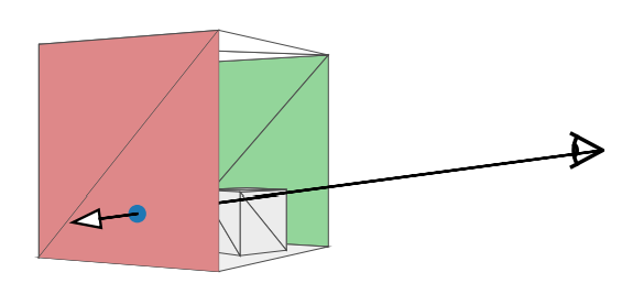
Ray trace the scene
Intersection - Ray vs Triangle
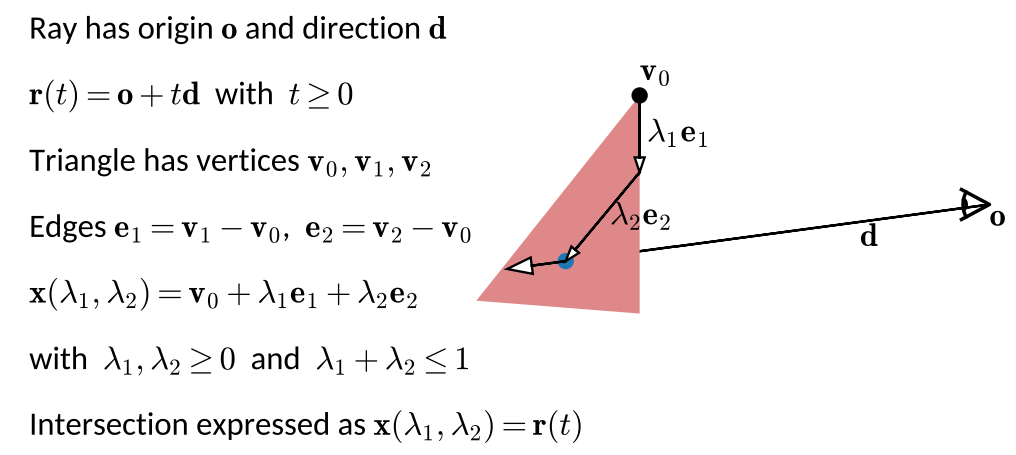
Use barycentric coordinate to describe point on the triangle, and it is equal to the point on the ray, it indicates an intersection.
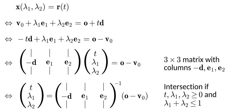
A mathmatic representation is as followed, and the goal here is to fomulate it toward getting the ray and 2 barycentric parameters.
// Checks whether a ray intersects a triangle
// \param out_t The ray parameter at the intersection (if any) (t)
// \param origin The position at which the ray starts (o)
// \param direction The direction vector of the ray (d)
// \param tri The triangle for which to check an intersection
// \return true if there is an intersection, false otherwise
bool ray_triangle_intersection(out float out_t, vec3 origin, vec3 direction, triangle_t tri) {
    vec3 v0 = tri.positions[0];
    mat3 matrix = mat3(-direction, tri.positions[1] - v0, tri.positions[2] - v0);
    vec3 solution = inverse(matrix) * (origin - v0);
    out_t = solution.x;
    vec2 barys = solution.yz;
    return out_t >= 0.0 && barys.x >= 0.0 && barys.y >= 0.0 && barys.x + barys.y <= 1.0;
}
Note that the function outputs are in 2 ways:
boolindicates the return value being a boolean, true if there is an intersection, false otherwiseout float out_tparameter indicate it will capture the ray parameter at the intersection (if any) (t), aka the hitting point
Intersection - Ray vs Mesh
// Checks whether a ray intersects any triangle of the mesh
// \param out_t The ray parameter at the closest intersection (if any) (t)
// \param out_tri The closest triangle that was intersected (if any)
// \param origin The position at which the ray starts (o)
// \param direction The direction vector of the ray (d)
// \return true if there is an intersection, false otherwise
bool ray_mesh_intersection(out float out_t, out triangle_t out_tri, vec3 origin, vec3 direction) {
    // Definition of the mesh geometry (exported from Blender)
    // ...

    // Find the nearest intersection across all triangles
    out_t = 1.0e38;
    for (int i = 0; i != TRIANGLE_COUNT; ++i) {
        float t;
        if (ray_triangle_intersection(t, origin, direction, tris[i]) && t < out_t) {
            out_t = t;
            out_tri = tris[i];
        }
    }
    return out_t < 1.0e38;
}
Note that the function outputs are in 3 ways:
boolindicates the return value, true if there is an intersection, false otherwiseout triangle_t out_tri: closest hit triangleout float out_t: ray parameter at the intersection (if smaller than max ray length)
On Path tracing
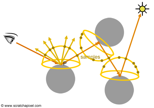
Global Illumination
Surfaces can be lit directly, but also indirectly, via paths of arbitrary length and directions.
Path tracing operation starts at camera, keep tracing done the bouncing rays (ray tracing) until finds a light source when it is lucky.
More from Scratchapixel
Global Illumination and Path Tracing
Radiance
$L_(x,w)$ is called radiance, which is basically color for the ray $x+tw$.
It is a plenoptic function / radiance field.
The plenoptic illumination function is an idealized function used in computer graphics to express the image of a scene from any possible viewing position at any viewing angle at any pointin time.
The final pixel color of the render result is the radiance for camera ray.
Radiance is constant along rays in vacuum. Which means if we trace a ray up from point $x$ to $y$, the radiance received at $x$ (from $y$) is the same as the radiance sent from $y$ (to $x$): $L(x,w)=L(y,-w)$
Ray tracing is transporting radiance, describes how light propogates in empty space.
Derivation of Radiance and other Rediometry Terms
Note: the best way is to follow the order of derivation of:
- Energy ($J$)
- flux ($W$)
- Irradiance and Radiant Exitance ($W/m^2$)
- Intensity ($W/sr$)
- Radiance ($W/m^2sr$)
It is well explained in pbrt but here we will follow the workshop structure.
More from pbrt
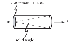
Radiance measures irradiance with respect to solid angles. Definition:
\[L = \frac{dE_{w}}{dw}\]where, $E_w$ is the irradiance at the surface that is perpendicular to the direction $w$:
\[E_{\omega} = \frac{d\phi}{dA^ \bot}\]so:
\[L = \frac{dE_w}{dw} = \frac{d^2 \phi}{d\omega \cdot dA^ \bot}\]which means, radiance is the flux density per unit area, per unit solid angle.
It is the limit of the measurement of incident light at the surface, as a cone of incident directions of interest dw becomes very small, and as the local area of interest on the surface dA also becomes very small.
Irradiance
We don’t just have to deal with empty space, we also have to figure out how light interact with the surface - this is defined by irradiance.
Irradiance is the weighted integral over radiance:
\[E(x,n(x)) = \int_{\Omega(x)}(L(x,w) n(x) \cdot w dw)\]More from pbrt
From a differential perspective, irradiance is the average density of power (flux, $\phi$) over the area ($A$). Taking the limit of differential power per differential area at a point p, we got Irradiance at point p:
\[E(p) = \frac{d\phi(p)}{dA}\]It is following Lambert’s cosine law.
Rendering Equation
*Note: this is the over simplified version for the workshop, more at this post:
\[L_o(x) = L{e}(x) + \frac{a(x)}{\pi} \int_{\Omega(x)}(L(x,w) n(x) \cdot w dw)\]- result: outgoing radiance $L_o(x)$ for diffuse surface at x
- compute incoming irradiance $E(x,n(x))=\int_{\Omega(x)}L(x,w) n(x) \cdot w dw$, aka. total light reaching x
- multiply by surface color $a(x)$ (this is actually albedo)
- divide by $\pi$ to ensure energy conservation (this is actually the diffuse BRDF)
- add light emitted at x, 0 if x is not a light source
Note: here is a good read about Albedo and Diffuse BRDF
Now we have to integrate over $\Omega(x)$, which contains infinite many of incoming direction vectors. Then, we need $L(x,w)$ for each integral, which equals to $L_o(y)$ where $y = ray_intersection(x,w) = x + tw$, and accordingly there are infinite many of point $y$.
Monte Carlo Integration
Monte Carlo Integration is the method we use to solve the rendering equation.
If we try picking(or sampling) ray direction $w_1$ at random, we have:
\[\int_{\Omega(x)}(L(x,w) n(x) \cdot w dw) \approx 2{\pi}L(x,w_1) n(x) \cdot w_1\]and when we sample for many (towards infinite) times:
\[\int_{\Omega(x)}(L(x,w) n(x) \cdot w dw) \approx 2{\pi} \frac{1}{N}\underset{j = 1}{\overset{N}{\sum }} L(x,w_j) n(x) \cdot w_j\]This is called a Monte Carlo Estimator, and when $N$ (the sampling times) approaches infinity, the estimate is approaching 100% probability on being the correct answer.
The errors of the estimator is called zero-mean noise.
I will document the derivations of Monte Carlo in another post as it is such an important field in pace tracing implementation. Also I have to brush up probability theories for that…
More from Scratchapixel
More from pbrt
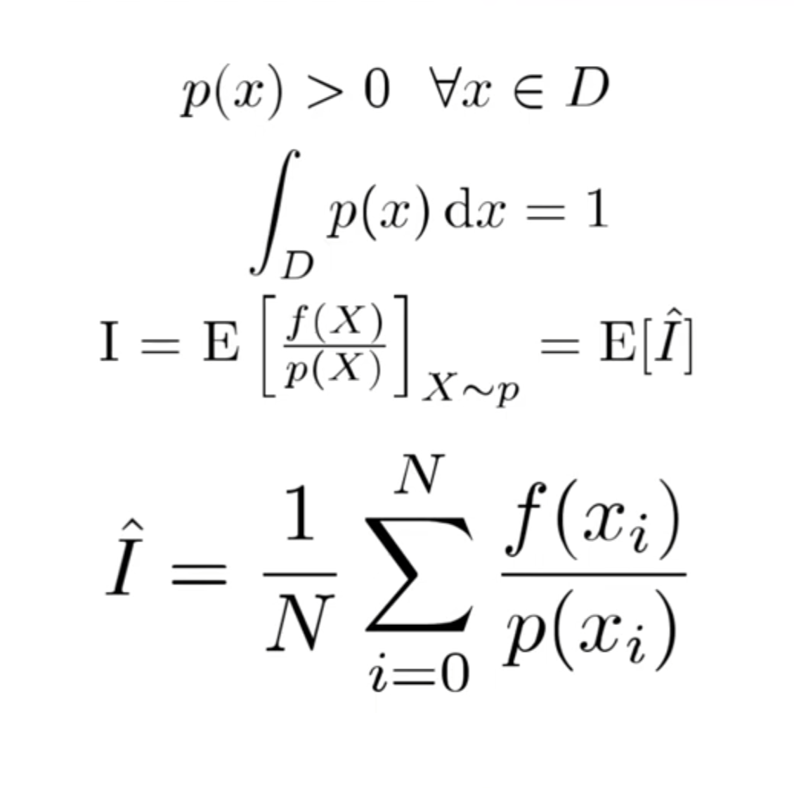
The expected value $E_p[f(x)]$ of a function $f$ is defined as the average value of the function over some distribution $p(x)$ over its domain $D$. Definition:
\[E_p[f(x)]=\int_D f(x)p(x)dx\]Given a supply of independent uniform random variable $X_i \in [a,b]$, the Monte Carlo Estimator is saying:
the expected value $E[F_n]$ of the estimator $F_n = \frac{b-a}{n} {\overset{n}{\underset{i=1}\sum}} f(X_i)$ is equal to the integral.
Here the uniform random variable is from a uniform distribution which has PDF of $p_{uniform}=\frac{1}{b-a}$, so the estimator can be written as
\[F_n = \frac{1}{n} {\overset{n}{\underset{i=1}\sum}} \frac{f(X_i)}{1/(b-a)} = \frac{1}{n} {\overset{n}{\underset{i=1}\sum}} \frac{f(X_i)}{p_{uniform}}\]Basically, $X_i$ can be drawn from any PDF $p(x)$, then the estimator is:
\[F_n = \frac{1}{n} {\overset{n}{\underset{i=1}\sum}} \frac{f(X_i)}{p(X_i)}\]then we have:
\[E[F_n] = E[\frac{1}{n} {\overset{n}{\underset{i=1}\sum}} \frac{f(X_i)}{p(X_i)}] = \frac{1}{n}{\overset{n}{\underset{i=1}\sum}} E[ \frac{f(X_i)}{p(X_i)}] = \frac{1}{n}{\overset{n}{\underset{i=1}\sum}}\int_D \frac{f(x)}{p(x)}p(x)dx\] \[= \int_D f(x)dx\]Final form of Monte Carlo Estimator in its full glory:
Uniform hemisphere sampling
Utility funtions to generate random direction vectors on hemisphere. It is using a uniform distribution to generate random numbers and map them to a random direction vector.
Code:
// Given uniform random numbers u_0, u_1 in [0,1)^2, this function returns a
// uniformly distributed point on the unit sphere (i.e. a random direction)
// (omega)
vec3 sample_sphere(vec2 random_numbers) {
    float z = 2.0 * random_numbers[1] - 1.0;
    float phi = 2.0 * M_PI * random_numbers[0];
    float x = cos(phi) * sqrt(1.0 - z * z);
    float y = sin(phi) * sqrt(1.0 - z * z);
    return vec3(x, y, z);
}


// Like sample_sphere() but only samples the hemisphere where the dot product
// with the given normal (n) is >= 0
vec3 sample_hemisphere(vec2 random_numbers, vec3 normal) {
    vec3 direction = sample_sphere(random_numbers);
    if (dot(normal, direction) < 0.0)
        direction -= 2.0 * dot(normal, direction) * normal;
    return direction;
}
Psendorandom number generator
// A pseudo-random number generator
// \param seed Numbers that are different for each invocation. Gets updated so
//             that it can be reused.
// \return Two independent, uniform, pseudo-random numbers in [0,1) (u_0, u_1)
vec2 get_random_numbers(inout uvec2 seed) {
    // This is PCG2D: https://jcgt.org/published/0009/03/02/
    seed = 1664525u * seed + 1013904223u;
    seed.x += 1664525u * seed.y;
    seed.y += 1664525u * seed.x;
    seed ^= (seed >> 16u);
    seed.x += 1664525u * seed.y;
    seed.y += 1664525u * seed.x;
    seed ^= (seed >> 16u);
    // Convert to float. The constant here is 2^-32.
    return vec2(seed) * 2.32830643654e-10;
}

// ...
// Use a different seed for each pixel and each frame
uvec2 seed = uvec2(pixel_coord) ^ uvec2(iFrame << 16, iFrame << 16 + 237);

// This gives 2 uniform random numbers in [0,1)
vec2 rands_0 = get_random_numbers(seed);
// These are different random numbers because seed has changed
vec2 rands_1 = get_random_numbers(seed);
Direct Illumination
Rendering direct illumination is the first step to test the theory - it only accounts for emission from light sources and direct illumination that from the light sources.
\[L(x) = L_e + \frac{a(x)}{\pi} \cdot 2{\pi} \cdot L_e(y) \cdot n(x) \cdot w\] \[y = ray\_intersection(x,w) = x + tw\]Direct + Indirect Illumination = GI!
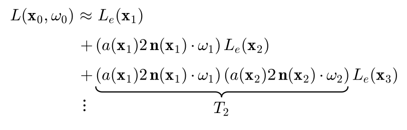
With camera ray $x_0, w_0$, we want to estimate $L(x_0, w_0)$ where
\[x_1 = ray\_intersection(x_0,w_0)\]Setting Monte Carlo $N = 1$, with a random direction $w_1$, we have:
\[L(x_0, w_0) = L_o(x_1) \approx L_e(x_1) + \frac{a(x_1)}{\pi} 2{\pi} L(x_1,w_1)n(x_1) \cdot w_1\]then from point $x_1$, ray trace to another random direction for next intersection point, and we will have:
\[x_2 = ray\_intersection(x_1,w_1)\] \[L(x_1, w_1) = L_o(x_2) \approx L_e(x_2) + \frac{a(x_2)}{\pi} 2{\pi} L(x_2,w_2)n(x_2) \cdot w_2\]and this keeps propagating… Path tracing is a recursion!
Flatten recursion into loop
Notice $\pi$ got cancelled out.
The process is now simplified into: in each iteration, add emission and update throughput weight $T_j$:
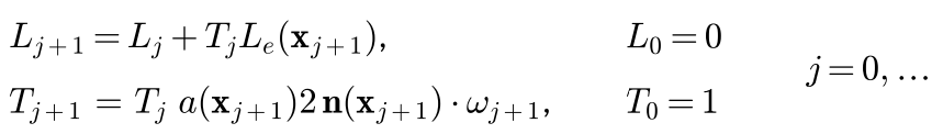
The function now is taking in a ray - a camera ray $(x_0, w_0)$. In a for-loop with MAX_PATH_LENGTH to control the ray tracing depth.
In the loop, we: trace next intersecting point and update to use it as the next ray trace origin; gather $T \cdot L_e$ into the radiance; sample a random direction to use it as the next ray trace direction; update throughput weight by multiplying it with
\[a(x_{j+1}) \cdot 2\cdot (n(x_{j+1}) \cdot w_{j+1})\]which is basically the aggragation of BRDF information AND the Monte Carlo factor of dividing the pdf
Note that, $1/\pi$ from BRDF and $\frac{1}{1/(2\pi)}$ from Monte Carlo multiply into 2.
// Performs path tracing: It starts with the given ray. If this ray intersects
// a triangle, a new random ray is traced iteratively, up to a fixed limit.
// \param origin The position at which the ray starts (x_j)
// \param direction The direction vector of the ray (omega_j)
// \param seed Needed for get_random_numbers()
// \return A noisy estimate of the reflected and emitted radiance at the point
//         intersected by the ray (i.e. the color) (L_o(x))
vec3 get_ray_radiance(vec3 origin, vec3 direction, inout uvec2 seed) {
    vec3 radiance = vec3(0.0);
    vec3 throughput_weight = vec3(1.0);
    for (int i = 0; i != MAX_PATH_LENGTH; ++i) {
        float t;
        triangle_t tri;
        if (ray_mesh_intersection(t, tri, origin, direction)) {
            radiance += throughput_weight * tri.emission;
            origin += t * direction;
            direction = sample_hemisphere(get_random_numbers(seed), tri.normal);
            throughput_weight *= tri.color * 2.0 * dot(tri.normal, direction);
        }
        else
            break;
    }
    return radiance;
}
The calling function. Remember to divide total radiance by sample amount N.
void mainImage(out vec4 out_color, in vec2 pixel_coord) {
    // Define the camera position and the view plane
    // Compute the camera ray
    // Use a different seed for each pixel and each frame

    // Perform path tracing with SAMPLE_COUNT paths
    out_color.rgb = vec3(0.0);
    for (int i = 0; i != SAMPLE_COUNT; ++i)
        out_color.rgb += get_ray_radiance(camera_position, ray_direction, seed);
    out_color.rgb /= float(SAMPLE_COUNT);
    // ...
}
Progressive rendering on Shadertoy
On shadertoy, we do everything in Buffer A, where out vec4 out_color is output into iChannel0. iChannel0 kept being sampled as prev_color and got added with newly sampled radiance weighted by per-frame contribution weight.
vec3 prev_color = texture(iChannel0, tex_coord).rgb;
float weight = 1.0 / float(iFrame + 1);
out_color.rgb = (1.0 - weight) * prev_color + weight * out_color.rgb;
out_color.a = 1.0;
In Image, we simply just display iChannel0 texture to full screen:
// Interesting things happen in Buffer A, this just displays the image
void mainImage(out vec4 out_color, in vec2 pixel_coord) {
    out_color = texture(iChannel0, pixel_coord / iResolution.xy);
}
Now we have the final result:
Final Thoughts
My journey into ray tracing began with Ray Tracing in One Weekend and then I dove into pbrt. Exploring pbrt constantly pushed me out of my comfort zone, urging me to dig deeper into its scientific and mathematical roots in path tracing and physically based rendering (pbr). This journey echoed my university days studying digital media and computer science—learning C++ programming, data structures, calculus, discrete math, probability theories, digital image processing, 3D art production, and more. Bringing these old concepts back with newfound relevance has been really rewarding :)
I’m thankful to this workshop for helping me tie together all my reading and research. Big shout-out to the author, Christoph Peters.
Even though I work as a Technical Artist focusing on game development and real-time production for film and animation, I’ve always been drawn to the detailed world of graphics engineering and low-level rendering theories. Exploring this field purely out of interest has proven incredibly beneficial for my role.
END