Finish reading Ray Tracing in One Weekend Chapter 2 to 6. Breakdown topics about raytracing analogy, simple camera model implementation, surface normal visualization, and Multisampling Antialiasing (MSAA) implementation.

Raytracing Overview

Light Rays (photons) are emitted from/bounced by/passing through the objects, and some of them made their way to arrive our eye retina/camera film to form the image we see/capture.

To reverse-engineer this, imaging from view origin (camera/eye position) we are shooting(emitting) View Rays through every pixel to “scan” the objects we are trying to render/see, and then gather the hit points to color the corresponding pixels.

…The core of a raytracer is to send rays through pixels and compute what color is seen in the direction of those rays. This is of the form calculate which ray goes from the eye to a pixel, compute what that ray intersects, and compute a color for that intersection point.

Image from - Scratchapixel 2.0

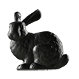
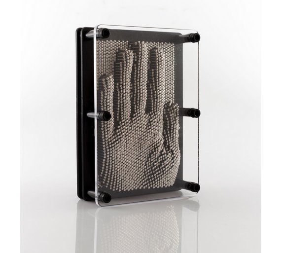
Even a better analogy for this process, I think, would be this kind of pin-art toy:

Draw with Ray

Simple Camera Model

The variation of the camera ray directions (one per pixel) form a “view volume/cone” - the view frustum, and every single ray provides a color value to its corresponding pixel to form the final image on a “film/retina” - the near clipping plane.

Image from - Scratchapixel 2.0

So, to draw an image with raytracing, we need to:

1. Set a range of the directions of the camera rays. This define the size of the screen.
2. Set color value for the pixel of every rays. (for higher rendering quality we can shoot multiple rays per pixel and average the coloration for that pixel.)

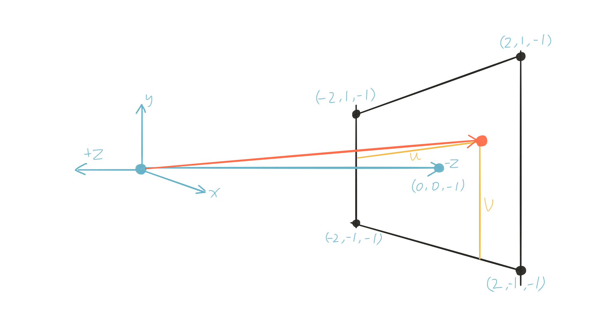
In order to respect the convention of a right-handed coordinate system, the negative z-axis is pointing into the screen (or, z-axis point out of screen).

For right-handed coordinates your right thumb points along the Z axis in the positive direction and the curl of your fingers represents a motion from the first or X axis to the second or Y axis. When viewed from the top or Z axis the system is counter-clockwise.

Image from - Wikipedia

Here we set the near clipping plane at -1 on the z-axis, and define the size of the screen with range from -2 to 2 on x-axis , and from -1 to 1 on y-axis.

class camera {
public:
    camera() {
        lower_left_corner = vec3(-2.0,-1.0,-1.0);
        horizontal = vec3(4.0,0.0,0.0); // horizontal range
        vertical = vec3(0.0,2.0,0.0);   // vertical range
        origin = vec3(0.0,0.0,0.0);
    }

    ray get_ray(float u, float v){return ray(origin, lower_left_corner + u*horizontal + v* vertical - origin);}

    vec3 lower_left_corner;
    vec3 horizontal;
    vec3 vertical;
    vec3 origin;
};

And we can build the camera rays with camera position and the pixel positions on the clipping plane. After we have the rays, we can use it to trace the scene and produce color values to draw the final image.

Camera Model

// pixel amount on x and y axis
int nx = 200;
int ny = 100;

camera cam;

for (int j = ny-1; j >= 0; j--)
{
    for (int i = 0; i < nx; i++)
    {
        vec3 col(0,0,0);

        float u = float(i) / float(nx);
        float v = float(j) / float(ny);

        ray r = cam.get_ray(u,v);
        vec3 p = r.point_at_parameter(1.0);
        p = unit_vector(p);
        col = vec3(p.z(),p.z(),p.z());

        int ir = int (255.99*col[0]);
        int ig = int (255.99*col[1]);
        int ib = int (255.99*col[2]);
    }
}

Color with depth values of normalized camera rays.

Draw Sphere

Details about ray-sphere intersection was documented in this previous post.

bool hit_sphere(const vec3& center, float radius, const ray& r) {
    vec3 oc = r.origin() - center;
    float a = dot(r.direction(), r.direction());
    float b = 2.0 * dot(oc, r.direction());
    float c = dot(oc,oc) - radius*radius;
    float discriminant = b*b - 4*a*c;
    return (discriminant>0);
}

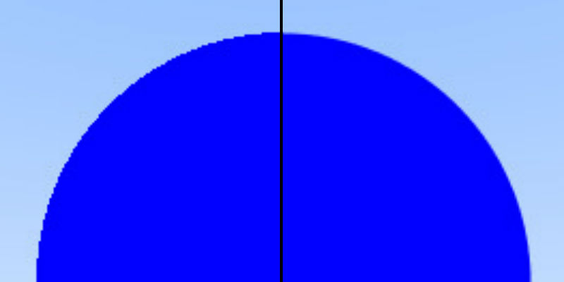
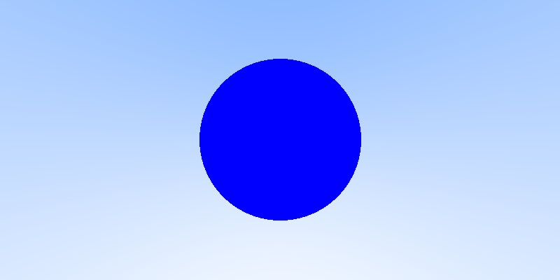
vec3 color(const ray& r) {
    // draw blue sphere
    if(hit_sphere(vec3(0,0,-1), 0.5, r))
        return vec3(0,0,1);

    // draw background, here we are drawing a gradient
    vec3 unit_direction = unit_vector(r.direction());
    float t = 0.5*(unit_direction.y()+1.0); // -1~1 --> 0~1
    return (1.0-t)*vec3(1.0,1.0,1.0) + t*vec3(0.5,0.7,1.0); // lerp
}

int main() {
    int nx = 200;
    int ny = 100;

    camera cam;

    for (int j = ny-1; j >= 0; j--) {
        for (int i = 0; i < nx; i++) {
            vec3 col(0,0,0);

            float u = float(i) / float(nx);
            float v = float(j) / float(ny);
            ray r = cam.get_ray(u,v);
            vec3 col = color(r);

            int ir = int (255.99*col[0]);
            int ig = int (255.99*col[1]);
            int ib = int (255.99*col[2]);
        }
    }
}

blended_value = (1-t)*start_value + t*end_value is using linear interpolation to create a gradient background.

Draw a sphere with raytracing and color it blue, along with background gradient.

Surface Normal Visualization

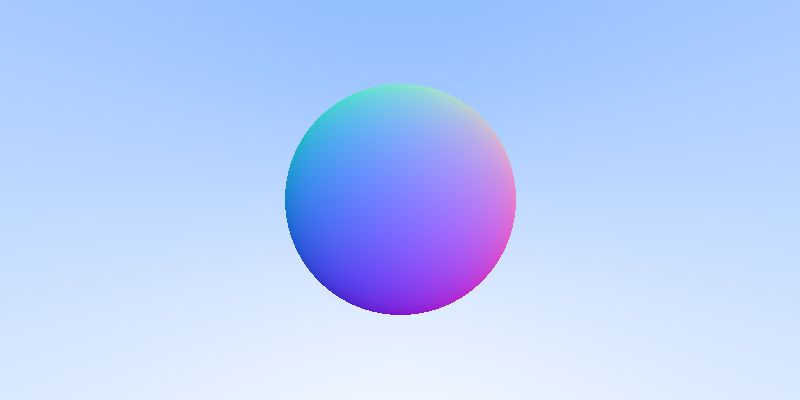
Without a proper shading, it is hard to say the blue disc we just drew is a sphere. To get a better sense of 3D, we can first of all visualize the surface normal of the sphere.

First of all we change the return value of hit_sphere() from bool to float, which is the intersecting distance. Explained also in previous post.

To calculate the surface normal of sphere at the hit point of the ray, simply calculate the vecter between sphere center and hit point and then normalize it. Here in code representation will be vec3 N = unit_vector(r.point_at_parameter(t) - vec3(0,0,-1)); where r.point_at_parameter(t) returns the hit point position and vec3(0,0,-1) is the sphere center.

Image from - Scratchapixel 2.0

float hit_sphere(const vec3& center, float radius, const ray& r){
    vec3 oc = r.origin() - center;
    float a = dot(r.direction(), r.direction());
    float b = 2.0 * dot(oc, r.direction());
    float c = dot(oc,oc) - radius*radius;
    float discriminant = b*b - 4*a*c;
    if(discriminant < 0){
        return -1.0;
    }
    else{
        return (-b - sqrt(discriminant)) / (2.0*a);
    }
}

vec3 color(const ray&r){
    // draw blue sphere
    float t = hit_sphere(vec3(0,0,-1), 0.5, r);
    if(t > 0.0){
        vec3 N = unit_vector(r.point_at_parameter(t) - vec3(0,0,-1));
        return 0.5*vec3(N.x()+1, N.y()+1, N.z()+1);
    }

    // draw background, here we are drawing a gradient
    ...
}

After mapping the normal vector to RGB color values by 0.5*vec3(N.x()+1, N.y()+1, N.z()+1);, we get the image like this:

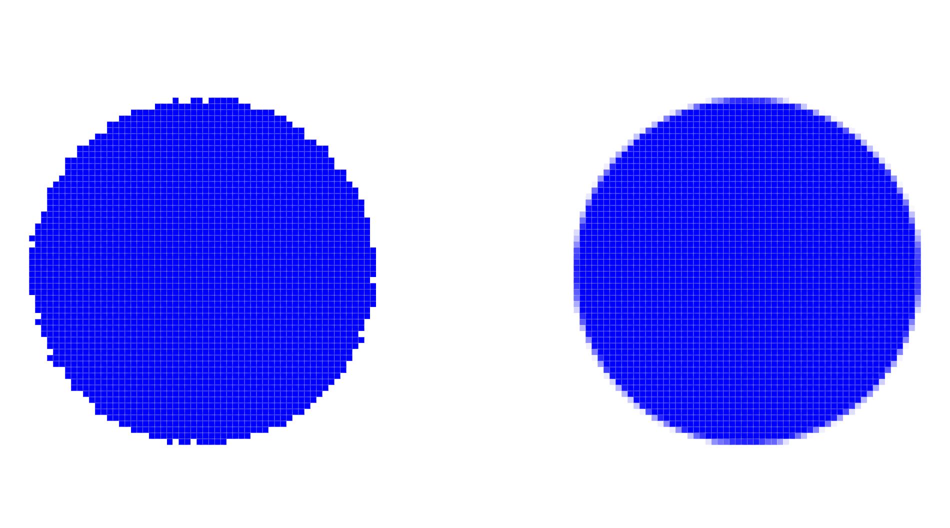
Multisampling Antialiasing

We have been assigning single color value for every single pixel. This causes bad aliasing effect in the final image.

Solution is to randomly shoot multiple camera rays per pixel and get multiple hit result for coloration. The amount of random rays is Sample Rate. Then we add up all the various color values for this pixel and divide it by sample rate to average the final color. This color would be much more representative than the color provided by only one ray.

Image from - SideFX Docs

int nx = 200;
int ny = 100;
int ns = 100;

camera cam;

for(int j=ny-1; j>=0; j--){
    for(int i=0; i<nx; i++){
        vec3 col(0,0,0);
        for(int s=0; s < ns; s++){
            float u = float(i + drand48())/float(nx); // 0~1
            float v = float(j + drand48())/float(ny);
            ray r = cam.get_ray(u,v);
            col += color(r);
        }
        col /= float(ns);

        int ir = int(255.99*col[0]);
        int ig = int(255.99*col[1]);
        int ib = int(255.99*col[2]);
    }
}

w/o and w/ MSAA