This post is the second part of my study notes on breaking down yumcyawiz’s project glsl330-cornellbox. This time will focus on the shader side of the renderer and look into the real implementation of path tracing in GLSL.
- Overview
- Vertex shader
rect.vert - Fragment shader
pt.frag - Output shader
- Ray generation
raygen.frag - BRDF sampling
brdf.frag - Final thoughts
Overview
The author breaks the shaders into multiple small bite pieces and have them included into the main shader. This makes the implementation very structured and it is even closely assemble the architecture of PBRT, which helped me a lot to have a bird’s eyes view of the system.
Vertex shader rect.vert
rect.vert is the only vertex shader needed in the application to process the quad mesh to be displayed on the screen.
#version 330 core
layout (location = 0) in vec3 vPos;
layout (location = 1) in vec2 vtexCoord;

out vec2 texCoord;

void main() {
  texCoord = vtexCoord;
  gl_Position = vec4(vPos, 1.0);
}
It defined 2 input vertex attributes to receive data from CPU on vertex positions and vertex texture coordinates (UV). Vertex positions are sent into gl_position in shader and UV is passed down the pipeline to fragment shader stage by using out keyword.
The data preparation (initialization) is done in rectangle.h in constructor Rectangle(). That includes:
- create and bind vertex array object
VAO, which stores instruction of how to use vertex data - create and bind vertex buffer object
VBO, which stores the real vertices data that being sent to GPU’s memory – copy vertices array into the buffer (VBO) for OpenGL to use (glBufferData) - create and bind element buffer object
EBO, which stores vertex indices - lastly set vertex attributes pointers (
glVertexAttribPointer)
and the drawing is done in Rectangle::draw() by:
- activate shader program
- bind VAO
- draw elements
- unbind VAO
- deactivate shader program
More details to refresh all the basic concepts at Hello Triangle - learnopengl.com
Fragment shader pt.frag
Overview and main() function
This is the main shader contains function computeRadiance(in Ray ray_in) that calculate the path tracing result.
It includes many other shader files:
global.fragthat contains definition of math constants and useful structs -PI;Ray,IntersectInfo,Material,Primitive,Light, etc.uniform.fragthat contains uniform variables and uniform blocks definition -accumTexture,stateTexture,GlobalBlock,CameraBlock,SceneBlock, etc.- note the uniform data types used:
- sampler2D for regular texture
- usampler2D for random state texture
- layout(std140) for uniform blocks
- note the uniform data types used:
uniform sampler2D accumTexture;
uniform usampler2D stateTexture;

layout(std140) uniform GlobalBlock {
  uvec2 resolution;
  float resolutionYInv;
};

layout(std140) uniform CameraBlock {
  vec3 camPos;
  vec3 camForward;
  vec3 camRight;
  vec3 camUp;
  float a;
} camera;

const int MAX_N_MATERIALS = 100;
const int MAX_N_PRIMITIVES = 100;
const int MAX_N_LIGHTS = 100;

layout(std140) uniform SceneBlock {
  int n_materials;
  int n_primitives;
  int n_lights;
  Material materials[MAX_N_MATERIALS];
  Primitive primitives[MAX_N_PRIMITIVES];
  Light lights[MAX_N_LIGHTS];
};
rng.fragfor random number generators and related functionsuint xorshift32(inout XORShift32_state state)float random()- return random float number between 0, 1
void setSeed(in vec2 uv)- sample the random state texture and use the value as the random number generator seed for each pixel/texel
raygen.fragto generate camera rayRay rayGen()
util.fragfor matrix transformationsfloat atan2()vec3 worldToLocal()vec3 localToWorld()
intersect.fragto define functions to check geometry intersectionbool intersectSphere()bool intersectPlane()
closest_hit.fragadded one layer of encapsulation for checking intersection for all primitives in the scenebool intersect_each()bool intersect()
sampling.fragto define functions to sample points on various surfacesvec3 sampleHemisphere()vec3 sampleCosineHemisphere()vec3 samplePlane()vec3 sampleSphere()vec3 samplePointOnPrimitive()
brdf.fragto define surface materialsfloat fresnel()vec3 BRDF()vec3 sampleBRDF()
These functions will be broken down later where necessary.
Shader started at main() function.
void main() {
    // set RNG seed
    setSeed(texCoord);

    // generate initial ray
    vec2 uv = (2.0*(gl_FragCoord.xy + vec2(random(), random())) - resolution) * resolutionYInv;
    uv.y = -uv.y;
    float pdf;
    Ray ray = rayGen(uv, pdf);
    float cos_term = dot(camera.camForward, ray.direction);

    // accumulate sampled color on accumTexture
    vec3 radiance = computeRadiance(ray) / pdf;
    color = texture(accumTexture, texCoord).xyz + radiance * cos_term;

    // save RNG state on stateTexture
    state = RNG_STATE.a;
}
It receives UV texCoord passed down by vertex shader; it also defines 2 uniform attributes for output:
in vec2 texCoord;

layout (location = 0) out vec3 color;
layout (location = 1) out uint state;
On CPU side, the 2 uniform are set by
// set uniforms
pt_shader.setUniformTexture("accumTexture", accumTexture, 0);
pt_shader.setUniformTexture("stateTexture", stateTexture, 1);
Inside the main function, it firstly calls setSeed(texCoord) feeding in screen quad UV to sample the stateTexture.
void setSeed(in vec2 uv) {
    RNG_STATE.a = texture(stateTexture, uv).x;
}
XORShift32_state RNG_STATE is defined in global.frag. It is set by setSeed() by sampling a stateTexture. stateTexture is a texture uniform passed in from CPU. It was initially setup in Renderer() in renderer.h with uniform_int_distribution.
In the end the random value is saved back to stateTexture (of each texel).
UV on the camera plane is calculated relative to the defined resolution, and flipped on y axis.
Camera ray is generated by rayGen(uv, pdf). pdf is filled with probability weight of the generated ray. (more explanation in following Ray generation section)
Computed radiance value then divides pdf from ray generation, and added into the accumTexture value, after scaled by cosine term (*pending explanation).
Compute radiance function
This code is using the similar approach from Notes from A Path Tracing Workshop since they both implement path tracing in GLSL shader code that do not support recursion.
First, it initializes couple of variables to be tracked and updated during the process:
float russian_roulette_prob = 1vec3 color = vec3(0)vec3 throughput = vec3(1)
Now entering main for-loop. It will loop till MAX_DEPTH.
vec3 computeRadiance(in Ray ray_in) {
    Ray ray = ray_in;

    float russian_roulette_prob = 1;
    vec3 color = vec3(0);
    vec3 throughput = vec3(1);

    for(int i = 0; i < MAX_DEPTH; ++i) {
        // ...
Russian Roulette
This is one of the new techniques incorporated in this implementation.
At the beginning of each loop, generate a random float between 0 and 1, if it is larger than russian_roulette_prob, break the loop aka terminate the path. If the loop is not broken, divide the throughput by russian_roulette_prob(which equals to scaling up the throughput).
if(random() >= russian_roulette_prob) {
    break; // this path ends here
}

throughput /= russian_roulette_prob;
At the end of each loop, if ray intersects the scene, after the throughput is updated, we get the max element of throughput (because it is a RGB value), and set that to be the newly updated russian_roulette_prob.
float throughput_max_element = max(max(throughput.x, throughput.y), throughput.z);

russian_roulette_prob = min(throughput_max_element, 1.0);
The theory behind it is better to understand heuristically. As the light keeps bouncing and the path keeps growing, the rarity of later bounces is growing continuously.
Here we are choosing russian_roulette_prob dynamically by computing it at each bounce according to possible color contribution, aka the throughput.
The more light bounces, the smaller the throughput, the smaller russian_roulette_prob will be set (min(throughput_max_element, 1.0)), and more possible that the random value drawn is larger than it then break the loop. When it didn’t break the loop, the division by russian_roulette_prob compensates the throughput for times where we miss the path.
Russian Roulette randomly terminates a path with a probability inversely equal to the throughput. So paths with low throughput that won’t contribute much to the scene are more likely to be terminated.
If we stop there, we’re still biased. We ‘lose’ the energy of the path we randomly terminate. To make it unbiased, we boost the energy of the non-terminated paths by their probability to be terminated. This, along with being random, makes Russian Roulette unbiased.
…In the end, Russian Roulette is a very simple algorithm that uses a very small amount of extra computational resources. In exchange, it can save a large amount of computational resources. source
Evaluate radiance
When ray intersects the scene, first get the hitPrimitive and hitMaterial from IntersectInfo struct.
if(intersect(ray, info)) {
    Primitive hitPrimitive = primitives[info.primID];
    Material hitMaterial = materials[hitPrimitive.material_id];
    // ...
If the hitMaterial emissive value is larger than 0, meaning it’s object is a light source and we will count its color into the final radiance contribution and terminate the path.
if(any(greaterThan(hitMaterial.le, vec3(0)))) {
    color += throughput * hitMaterial.le;
    break;
}
If the first hit object is NOT a light source, we continue tracing the next ray by sampling the BRDF of the hit surface.
Note that wo is the vector of bounced light leaving/heading outward of the surface, and wi is the vector of bounced light arriving/heading inward the surface. Hence the o and i subscripts. Since ray is shooting from the camera toward the scene that means wo is the opposite direction of ray:
wo also has to be transformed into surface local space to be used to evaluate BRDF.
vec3 wo = -ray.direction;
vec3 wo_local = worldToLocal(wo, info.dpdu, info.hitNormal, info.dpdv);
BRDF sampling:
// BRDF Sampling
float pdf;
vec3 wi_local;

// material contains type ID, kd, le emissive
vec3 brdf = sampleBRDF(wo_local, wi_local, hitMaterial, pdf);

// prevent NaN
if(pdf == 0.0) {
    break;
}

vec3 wi = localToWorld(wi_local, info.dpdu, info.hitNormal, info.dpdv);

// update throughput
float cos_term = abs(wi_local.y);
throughput *= brdf * (1 / pdf) * cos_term;

// update russian roulette probability
// ...
Here we can see throughput is scaled by
- BRDF
- sampling pdf, and
- surface cosine term
Note that the brdf sampling pdf is calculated inside the brdf shader file, as well as the bounced-off light direction in local space wi_local.
This direction, together with the hit point position, are later to be used to generate next ray.
// set next ray
ray = Ray(info.hitPos, wi);
In the end if ray is not intersecting anything, simply:
for(int i = 0; i < MAX_DEPTH; ++i) {
  // ...
  if(intersect(ray, info)) {
      //...
  } else {
      color += throughput * vec3(0);
      break;
  }
}
return color; // radiance
Comparing with the previous workshop GLSL code for evaluating radiance, notice the similarity:
vec3 get_ray_radiance(vec3 origin, vec3 direction, inout uvec2 seed) {
    // initial radiance and throughput
    vec3 radiance = vec3(0.0);
    vec3 throughput_weight = vec3(1.0);

    // main loop
    for (int i = 0; i != MAX_PATH_LENGTH; ++i) {

        float t;
        triangle_t tri;

        // if intersect with the scene, ray length and hit tri will be returned
        if (ray_mesh_intersection(t, tri, origin, direction)) {
            // count in emission
            radiance += throughput_weight * tri.emission;

            // move ray origin forward, as origin for next ray
            origin += t * direction;
            // randomly pick next ray direction
            direction = sample_hemisphere(get_random_numbers(seed), tri.normal);

            // update throughput
            throughput_weight *= tri.color * 2.0 * dot(tri.normal, direction);

        }
        else
            break;
    }
    return radiance;
}
Output shader
accumTexture is sampled at this stage and samplesInv uniform is passed in to normalize the result by dividing the sample amount.
#version 330 core

uniform float samplesInv;
uniform sampler2D accumTexture;

in vec2 texCoord;
out vec4 fragColor;

void main() {
  vec3 color = texture(accumTexture, texCoord).xyz * samplesInv;
  // gamma
  fragColor = vec4(pow(color, vec3(0.4545)), 1.0);
}
void render() {
    // ...
    switch (mode) {
        case RenderMode::Render:
        glBindFramebuffer(GL_FRAMEBUFFER, accumFBO);
        switch (integrator) {
            case Integrator::PT:
            rectangle.draw(pt_shader);
            break;
        }
        glBindFramebuffer(GL_FRAMEBUFFER, 0);

        // update samples
        samples++;

        // output
        output_shader.setUniform("samplesInv", 1.0f / samples);
        rectangle.draw(output_shader);
        break;

// ...
}
Ray generation raygen.frag
Here breakdown some details in camera ray generation function. Note that all camPos, camForward etc. vectors are passed in by CameraBlock uniform (located in uniform.frag).
Ray rayGen(in vec2 uv, out float pdf) {
    vec3 pinholePos = camPos + 1.7071067811865477 * camForward; //?
    vec3 sensorPos = camPos + uv.x * camRight + uv.y * camUp;

    Ray ray;
    ray.origin = camPos;
    ray.direction = normalize(pinholePos - sensorPos);
    float cosineTheta = dot(ray.direction, camForward);
    pdf = 1.0 / pow(cosineTheta, 3.0);
    return ray;
}
A pinhole camera:
The ray direction is picked by pointing from pixel position on the screen sensorPos to pinholePos. Here it seems the pinhole position is moved forward by a small amount(?) from the camera position. Sensor position is at camPos, so this way ray.direction = normalize(pinholePos - sensorPos) will guarantee the camera ray is shooting into the scene.
Interestingly, the generated camera ray here has a pdf as $\frac{1}{cos^3(\theta)}$ which confused me a lot.
After a long time research, I found some explanations:
From pbrt 5.4.1 The Camera Measurement Equation:
\[E(p,n)=\int_\Omega L_i(p,w) |cos\theta|dw_i \;\;\; (4.7)\] \[dw = \frac{ dA cos \theta} {r^2} \;\;\; (4.9)\]Given the incident radiance function, we can define the irradiance at a point on the film plane. If we start with the definition of irradiance in terms of radiance, Equation (4.7), we can then convert from an integral over solid angle to an integral over area using Equation (4.9).
The ratio between differential solid angle and differential area (4.9) is mentioned in PBRT at 4.2.3 Integrals over Area. In other words, radiance arriving on a point/small surface patch $dA$ (aka a pixel) is in proportion to the radiance arriving from a direction $dw$.
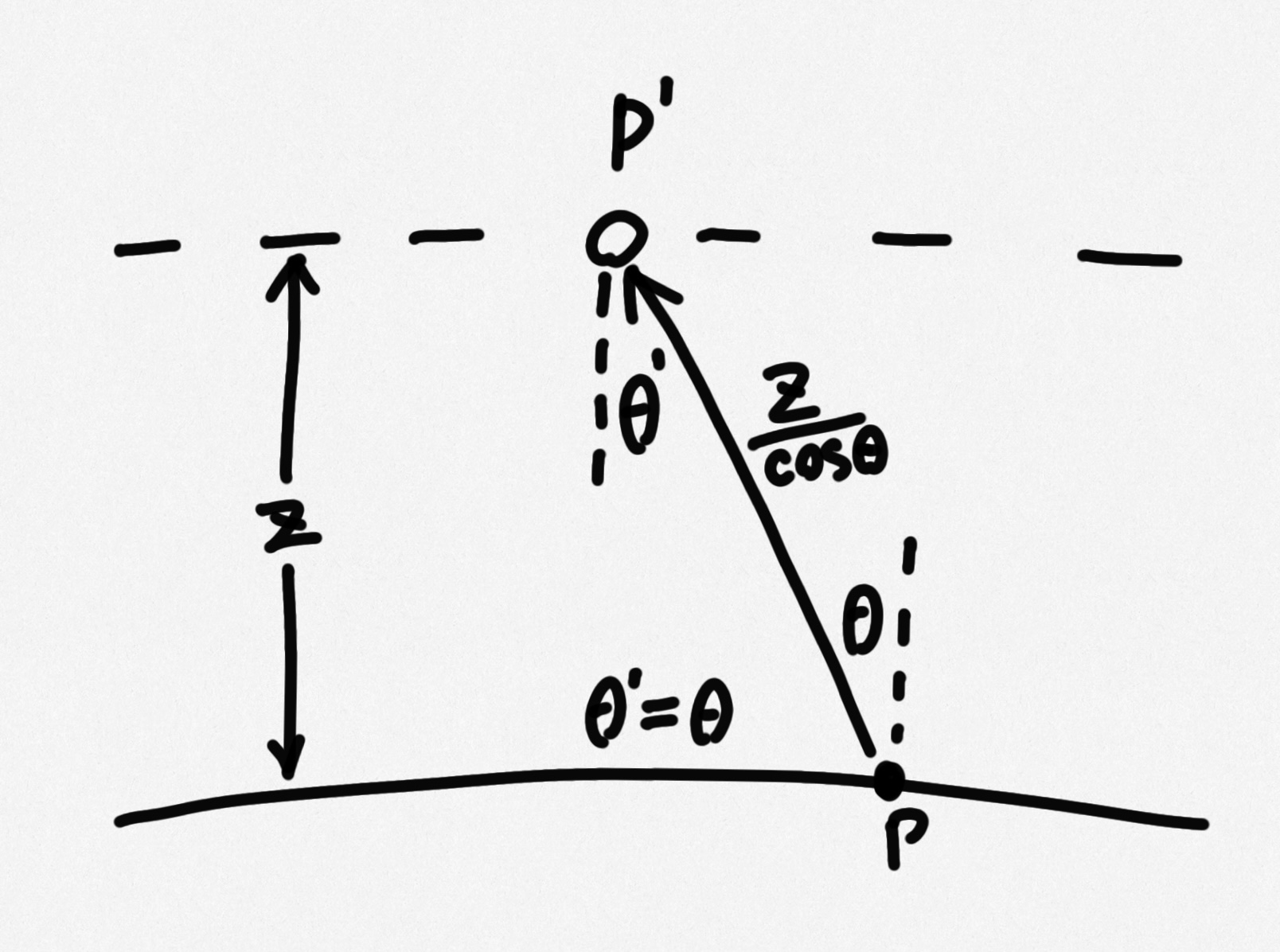
\[E(p) = \int_AL_i(p,p') \frac{|cos\theta'|}{\|p'-p\|^2} |cos\theta|dA\]This gives us the irradiance for a point on the film plane:
The perpendicular distance between the back of the lens (z coordinate of pinholePos for our case) and the film (z coordinate of sensorPos) is $z$, so $|p’-p| = \frac{z}{cos\theta}, \; \theta’ = \theta$ because:
put all together:
\[E(p) = \int_AL_i(p,p') \frac{|cos^3\theta|}{z^2} |cos\theta| dA\]More detailed explanation can refer to this amazing article Why You Weight Your Camera Rays the Way You Probably Did. And similar quote from Source:
GenerateRay returns a weight for the generated ray. The radiance incident along the ray from the scene is modulated by this weight before adding the contribution to the Film.
You will need to compute the correct weight to ensure that the irradiance estimate produced by pbrt is unbiased. That is, the expected value of the estimate is the actual value of the irradiance integral. Note that the weight depends upon the sampling scheme used.
Set $z = 1$ for the camera model:
For pinhole apertures, we compute the intersection with a plane arbitrarily set at to get a point along the ray leaving the camera before performing the projection. 16.1.1 Sampling Cameras
So the generated camera ray has a pdf of $\frac{1}{cos^3(\theta)}$ that the computed radiance have to divide; then the same cosine term have to multiply the radiance to get the real unbiased result, which in total is equivalent to multiply $cos^4(\theta)$:
void main() {
    // ...

    float pdf;
    Ray ray = rayGen(uv, pdf);
    float cos_term = dot(camForward, ray.direction);

    // accumulate sampled color on accumTexture
    vec3 radiance = computeRadiance(ray) / pdf;
    color = texture(accumTexture, texCoord).xyz + radiance * cos_term;

    // ...
}
More from 5.4.1 The Camera Measurement Equation:
For cameras where the extent of the film is relatively large with respect to the distance z, the $cos^4(\theta)$ term can meaningfully reduce the incident irradiance—this factor also contributes to vignetting.
… Although these factors apply to all of the camera models introduced in this chapter, they are only included in the implementation of the RealisticCamera. The reason is purely pragmatic: most renderers do not model this effect, so omitting it from the simpler camera models makes it easier to compare images rendered by pbrt with those rendered by other systems.
*This part took me a while to chase down a plausible explanation. May have to revist in the future.
BRDF sampling brdf.frag
The code separate the BRDF evaluation, and switches it by 3 classic material types - lambert, mirror and glass.
Note that the sampling of the lambert surface is also done here which will provides the corresponding pdf. The pdf will be passed outside into path tracing main loop and used for monte carlo estimation by dividing it.
It also outputs the bounced ray direction wi.
sampleCosineHemisphere(random(), random(), pdf) is in sampling.frag and is taking in random values from random() in rng.frag:
// sampling.frag
vec3 sampleCosineHemisphere(in float u, in float v, out float pdf) {
    float theta = 0.5 * acos(clamp(1.0 - 2.0 * u, -1.0, 1.0));
    float phi = 2.0 * PI * v;
    float y = cos(theta);
    pdf = y * PI_INV;
    return vec3(cos(phi) * sin(theta), y, sin(phi) * sin(theta));
}
The random function requires RNG_STATE, which is set by setSeed(texCoord) in main function, which samples the random state texture stateTexture. Since frag shader is running per each pixel, this will make each pixel has its unique seed.
// rng.frag
uint xorshift32(inout XORShift32_state state) {
    uint x = state.a;
    x ^= x << 13u;
    x ^= x >> 17u;
    x ^= x << 5u;
    state.a = x;
    return x;
}

float random() {
    return float(xorshift32(RNG_STATE)) * 2.3283064e-10;
}

void setSeed(in vec2 uv) {
    RNG_STATE.a = texture(stateTexture, uv).x;
}
material.kd here is the albedo of the lambert surface.
// brdf.frag
vec3 sampleBRDF(in vec3 wo, out vec3 wi, in Material material, out float pdf) {
    switch(material.brdf_type) {
    // lambert
    case 0:
        // receiving sample pdf
        // then pass back out to caller
        wi = sampleCosineHemisphere(random(), random(), pdf);
        // return albedo, kd kf
        return material.kd * PI_INV;
        break;

    // mirror
    case 1:
        pdf = 1.0;

        wi = reflect(-wo, vec3(0, 1, 0));
        return material.kd / abs(wi.y);
        break;

    // glass
    case 2:
        pdf = 1.0;

        // set appropriate normal and ior
        vec3 n = vec3(0, 1, 0);
        float ior1 = 1.0;
        float ior2 = 1.5;
        if(wo.y < 0.0) {
            n = vec3(0, -1, 0);
            ior1 = 1.5;
            ior2 = 1.0;
        }
        float eta = ior1 / ior2;

        // fresnel
        float fr = fresnel(wo, ior1, ior2);

        // reflection
        if(random() < fr) {
            wi = reflect(-wo, n);
        }
        // refract
        else {
            wi = refract(-wo, n, eta);
            // total reflection
            if(wi == vec3(0)) {
                wi = reflect(-wo, n);
            }
        }

        return material.kd / abs(wi.y);
        break;
    }
}
Final thoughts
By breaking down this project, I refreshed my basic OpenGL knowledge and revisited the GLSL path tracing workshop I previously covered. This project follows a similar implementation but incorporates additional optimization techniques, such as Russian Roulette. The shader code is well-organized and modular, mirroring the structure of PBRT. This project has integrated many of my learning resources. I plan to revisit the code and potentially extend it with more path tracing techniques or additional primitive/material support.
END