A post of all mathmatical descriptions and diagrams for rendering and path tracing theories that I found inspiring. Mainly based on the open courses Rendering (186.101, 2021S) by TU Wien, and few references to pbrt.
Light
Light integral over the hemisphere
- To sum up all the light, that is an integral.
- To sum up from all direction, that is a hemisphere
- light arriving at point $x$
- light from direction $w$ - by ray tracing
- differential solid angle $dw$
this is irradiance.

Irradiance integrates the total incident light over the hemisphere Ω and is measured in watts per meter squared [W · m −2 ].
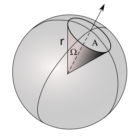
Solid angle
- Projected area on unit sphere.
- Full solid angle is $4\pi$.
- Hemisphere has solid angle of $2\pi$
Differential term conversion
Relationship between a surface patch and the solid angle:
\[dw = \frac{dAcos\theta}{r^2}\]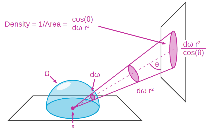
Light integral over the surface
Integrate over a single light surface:
\[L_i^{[l]}(x) = \int_{S_l} L_e^{[l]}(y) cos(\theta_x) \frac{cos\theta_y}{r^2} dA_y\]- light from source $[l]$ arriving at point $x$
- light intensity at position $y$ on the surface
where applied the conversion:
\[\frac{cos\theta_y}{r^2} dA_y = dw\]- $cos\theta_x$ is reveiver cosine
- $cos\theta_y$ is emitter cosine
Radiance
Radiance $L$ is flux per unit projected area per unit solid angle:
\[L = \frac{d\Phi}{dA^\perp dw}\]Radiance is a density over both space and angle.

- Sensors are sensitive to radiance
- It’s what you assign to pixels
- The fundamental quantity in image synthesis
- radiance stays constant along straight lines*
- All relevant quantities (irradiance, etc.) can be derived from radiance
BSDF
Recap irradiance:
\[L_i(x) = \int_\Omega L_i(x,w)cos(\theta_x)dw\]Now update integral to calculate how much light is going to the camera:
\[L_e(x,v) = \int_\Omega f_r(x, w \rightarrow v) L_i(x,w) cos(\theta_x) dw\]- $L_e(x,v)$ is exitant light going towards direction $v$ from point $x$
- light going in direction $v$ (the viewing direction)
- materials is modelled by BRDF $f_r$
how much light is reflected from a given direction into another given direction at a given position, and in which wavelengths
- light from direction $w$
- differential solid angle $dw$

Furnace test
White furnace test, energy conservation
(set $L_i$ to 1 and check $L_e \leq 1$)
… we can derive: $f_r$ of a white diffuse material is $1/\pi$
TBC
Rendering equation
Photons are emitted from light sources, reflected by surfaces in the scene until they reach the sensor. In rendering, we (can) go the opposite way. We trace importons until they reach a light source.
1. Recursive formulation
Recap light integral with BSDF:
\[L_e(x,v) = \int_\Omega f_r(x, w \rightarrow v) L_i(x,w) cos(\theta_x) dw\]It computes the light which is going into direction $v$, integrate over hemisphere, check all directions for incoming light, cosine weighting and material
Add light emittance, now we have recursive formulation:
\[L_e(x,v) = E(x,v) + \int_{\Omega} f_r(x,w \rightarrow v) L_i(x,w) cos(\theta_x) dw\]Expand the recursion
\[L(x_1 \rightarrow v) = E(x_1 \rightarrow v) + \int_{\Omega_1} f_r(x_1,w_1 \rightarrow v) L(x_1 \leftarrow w_1) cos(\theta_x) dw_1\] \[L(x_1 \rightarrow w_2) = E(x_2 \rightarrow w_2) + \int_{\Omega_2} f_r(x_2,w \rightarrow w_2) L(x_2 \leftarrow w) cos(\theta_x) dw\]where,
\[L(x_1 \leftarrow w_1) = L(x_1 \rightarrow w_2)\]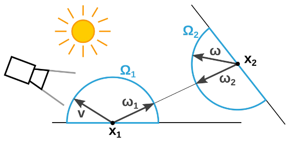
Generally:
\[L(x \rightarrow v) = E(x \rightarrow v) + \int_{\Omega} f_r(x,w \rightarrow v) L(x \leftarrow w) cos(\theta_x) dw\]2. Operator formulation
\[L = L_e + TL\]- T: light transport operator
-
K: local scattering operator, $L_o = KL_i$, turn incoming radiance into outgoing radiance, material
-
G: propagation operator, $L_i = GL_o$, turn outgoing radiance into incoming radiance, ray-tracing
- S: solution operator
This equation reaches an equilibrium after infinite time / iterations, after which it gives us the solution for the light distribution in the scene.
3. Path integral formulation
\[I_j = \int_\Omega f_j(\bar{x}) d_\mu(\bar{x})\]- $I_j$ is measurement for a sensor element aka pixel
- $\Omega$ is tje set of all transport paths at all lengths
- $f_j$ is measurement contribution function
- $\bar{x}$ is path between light source and sensor
- $\mu$ is measure on $\Omega$
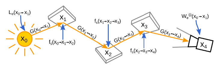
Expand the measurement contribution function:
\[f_j(\bar{x}) = L_e(x_0 \rightarrow x_1)\] \[G(x_0 \rightarrow x_1)f_s(x_0 \rightarrow x_1 \rightarrow x_2)\] \[G(x_1 \rightarrow x_2)f_s(x_1 \rightarrow x_2 \rightarrow x_3)\] \[... \; G(x_{k-1} \rightarrow x_k)W_e^{(j)}(x_{k-1} \rightarrow x_k)\]where,
\[G(x \leftrightarrow x') = V(x \leftrightarrow x') \frac{|cos(\theta_o)cos(\theta_i')|}{||x-x'||^2}\]$f_j$ is a product of several factors:
- the light emission $L_e$, which is simply the brightness of the light at position $x_0$
- the geometry factors between each pair of vertices – $G$
- the scattering factors $f_s$ for each inner vertex (reflection point), which model the material
- and finally the importance emission from the camera $W_e$.
So the path integral formulation is really just an integral which integrates over all surfaces at the same time.
\[I_j = \int_\Omega f_j(\bar{x}) d_\mu(\bar{x})\] \[= \int_{\Omega_0} f_j(\bar{x}) d_\mu(\bar{x}) \; + \; \int_{\Omega_1} f_j(\bar{x}) d_\mu(\bar{x}) \; + \; ... \; + \;\int_{\Omega_{\infty}} f_j(\bar{x}) d_\mu(\bar{x})\]More on pbrt:
Path tracing
Path tracing roadmap
- rendering equation recap
- direct lighting
- path tracing v0.5
- sample distribution
- russian roulette
- bsdf interface
- path tracing v1.0
Direct lighting
Start from recursive formulation for rendering equation:
\[L(x \rightarrow v) = E(x \rightarrow v) + \int_{\Omega} f_r(x,w \rightarrow v) L(x \leftarrow w) cos(\theta_x) dw\]Simplify notation:
-
$E(x \rightarrow v) \; to \; E_x$
-
$f(x,w \rightarrow v) \; to \; 1/\pi$
For direct lighting, stop after the first bounce.
Replace indefinite integral with Monte Carlo integral:
\[L(x \rightarrow v) = E_x + \frac{1}{N} \sum_{i=1}^N \left( \frac{1}{\pi} E_y \; cos(\theta_{\omega_i}) \frac{1}{p(w_i)} \right)\]Pull the sum out:
\[L(x \rightarrow v) = \frac{1}{N} \sum_{i=1}^N \left( E_x + \frac{1}{\pi} E_y \; cos(\theta_{\omega_i}) \frac{1}{p(w_i)} \right)\]Uniform hemisphere sampling
- For each $w$, draw 2 uniform random numbers $x1,x2$ in range $[0, 1)$
- Calculate $cos(\theta) = x_1, \; sin(\theta) = \sqrt{1−cos^2(\theta)}$
- Calculate $cos(\phi) = cos(2\pi x_2) , \; sin(\phi)=sin(2\pi x_2)$
- $w=Vector3(cos(\phi)sin(\theta),sin(\phi)sin(\theta),cos(\theta) )$
- $p(w) = \frac{1}{2\pi}$
Note that resulting $w$ is in local coordinate frame, z axis is normal to surface. To intersect scene, rays have to be in world space. Use coordinate transform between local and world.
Pseudocode:
for (i = 0; i < N; i++)
  v_inv = camera.gen_ray(px, py)
  x = scene.trace(v_inv)
  f = x.emit
  omega_i, prob_i = hemisphere_uniform_world(x)

  r = make_ray(x, omega_i)
  y = scene.trace(r)

  f = 1/pi * y.emit * dot(x.normal, omega_i) / prob_i

  pixel_color += f

pixel_color /= N
Indirect lighting
Start from recursive formulation for rendering equation:
\[L(x \rightarrow v) = E(x \rightarrow v) + \int_{\Omega} f_r(x,w \rightarrow v) L(x \leftarrow w) cos(\theta_x) dw\]Simplify notation:
-
$E(x \rightarrow v) \; to \; E_x$
-
$f(x,w \rightarrow v) \; to \; f_r$
then expand the recursive integral:
\[L(x \rightarrow v) = E_x + \int_\Omega f_r \; \left( E_{x'} + \int_{\Omega'} f_{r'} \; ... \; cos(\theta_{\omega'})dw' \right) \; cos(\theta_\omega)dw\]Turning into Monte Carlo integration:
\[L(x \rightarrow v) = E_x + \frac{1}{N} \sum_{i=1}^N f_r \; \left( E_{x'} + \frac{1}{N} \sum_{j=1}^N f_{r'} \; ... \; cos(\theta_{\omega_j'})\frac{1}{p(w_j')} \right) \; cos(\theta_{\omega_i})\frac{1}{p(w_i)}\]or collapse back:
\[L(x \rightarrow v) = E_x + \frac{1}{N} \sum_{i=1}^N f_r \; L(x \leftarrow w_i) \; cos(\theta_{\omega_i})\frac{1}{p(w_i)}\]Pseudocode:
v_inv = camera.gen_ray(px, py)
pixel_color = Li(v_inv, 0)

function Li(v_inv, D)
  if (D >= NUM_BOUNCES)
    return 0

  x = scene.trace(v_inv)
  f = 0

  for (i = 0; i < N; i++)
    omega_i, prob_i = hemisphere_uniform_world(x)
    ray = make_ray(x, omega_i)
    f += x.alb/pi * Li(ray, D+1) * dot(x.normal, omega_i) / prob_i

  return x.emit + f/N
Reconsider sample distribution
Flatten the integral
\[L(x \rightarrow v) = E_x + \int_\Omega f_r \; \left( E_{x'} + \int_{\Omega'} f_{r'} \; ... \; cos(\theta_{\omega'})dw' \right) \; cos(\theta_\omega)dw\]into:
\[L(x \rightarrow v) = E_x\] \[+ \int_\Omega f_r \; E_{x'} \; cos(\theta_\omega)dw\] \[+ \int_\Omega f_r \; \int_{\Omega'} f_r' \;\; E_{x''} \;\; cos(\theta_{\omega'})cos(\theta_w) \;\; dw'dw\] \[+ \int_\Omega f_r \; \int_{\Omega'} f_r' \; \int_{\Omega''} f_r'' \;\; E_{x'''} \;\; cos(\theta_{\omega''})cos(\theta_w')cos(\theta_w) \;\; dw''dw'dw\] \[+ ...\]Recap path integral form
Compare it with the path integral fomulation
\[I_j = \int_\Omega f_j(\bar{x}) d_\mu(\bar{x})\] \[= \int_{\Omega_0} f_j(\bar{x}) d_\mu(\bar{x}) \; + \; \int_{\Omega_1} f_j(\bar{x}) d_\mu(\bar{x}) \; + \; ... \; + \;\int_{\Omega_{\infty}} f_j(\bar{x}) d_\mu(\bar{x})\]The path integral form used a single integral for each bounce!
\[L(x \rightarrow v) = E_x\] \[+ \int_{\Omega_1} \; f_r \; E_{x'} \; cos(\theta_\omega) \; d\mu({\bar x})\] \[+ \int_{\Omega_2} \; f_r f_r' \; E_{x''} \; cos(\theta_{\omega'})cos(\theta_w) \; d\mu({\bar x})\] \[+ \int_{\Omega_3} \; f_r f_r' f_r'' \;\; E_{x'''} \;\; cos(\theta_{\omega''})cos(\theta_{\omega'})cos(\theta_w) \;\; d\mu({\bar x})\] \[+ ...\]Replace each integral with Monte Carlo integration
\[L(x \rightarrow v) = E_x\] \[+ \frac{1}{N} \sum_{i=1}^{N} \; f_r \; E_{x'} \; cos(\theta_\omega) \; \frac{1}{p(w)}\] \[+ \frac{1}{N} \sum_{i=1}^{N} \; f_r f_r' \; E_{x''} \; cos(\theta_{\omega'})cos(\theta_w) \; \frac{1}{p(w)p(w')}\] \[+ ...\]Pull the sum to the front, we achieve using a single sum for integration with recursion.
Pseudocode:
for (i = 0; i < N; i++)
  v_inv = camera.gen_ray(px, py)
  pixel_color += Li(v_inv, 0)
pixel_color /= N

function Li(v_inv, D)
  if (D >= NUM_BOUNCES)
    return 0

  x = scene.trace(v_inv)
  f = x.emit
  omega, prob = hemisphere_uniform_world(x)

  r = make_ray(x, omega)

  f += x.alb/pi * Li(r, D+1) * dot(x.normal, omega)/prob

  return f
END